Solution Analysis and Recommendations
Evaluating protocol changes requires understanding their potential impact. The complexity of liquidations makes this a high dimensional endeavor, so this section focuses on distilling it down to a few key metrics. The insights from that analysis point toward concrete solutions.
Impact Framing
The solution can follow a barbell approach to impact:
- If the change meaningfully improves protocol competitiveness and has high impact, it may warrant substantial resource allocation and a larger protocol upgrade
- If the impact is positive but limited, the focus should shift toward minimizing audit surface. In that case, the best approach is to pursue simple, low risk changes that capture whatever gains are available, even if small
To evaluate (1) compare against competitors. Empirical data lightly suggests that being the leader on capital efficiency has helped attract users, who are unlikely to migrate if Compound only raises CFs to the middle of the pack, especially with strong competition from protocols such as Aave, Morpho, Euler, and Fluid.
To determine (2) compare partial vs full liquidations.
Competitive impact of partial liquidations
Previously some analysis was posted comparing the capital efficiency of Compound III and Aave V3 using metrics such as insolvency buffer and liquidation collateral costs. This refreshes the previous analysis by incorporating partial liquidations.
Insolvency buffer derivation for partial liquidations
The first task is to update Gauntlet’s previous derivation of the IB to account for partial liquidations. Denote the close factor as c. From the protocol’s perspective, the collateral it holds now comes from both the portion absorbed and the remaining balance left in the account.
Let the amount of debt in the account be D and the collateral amount be C. In an absorption currently C(1-LP) is credited to the borrower’s debt balance so the amount of base asset given from the protocol to the borrower is given by \max(D, C(1-LP)). Generally, at the moment an account becomes liquidatable, D = C \cdot LF \leq C \cdot LF_{\max} = C(1-LP). This relationship matters especially for partial liquidations, where smaller liquidations may not exceed the borrower’s debt.
The protocol sale value of the absorbed collateral is c \cdot C(1-LP \cdot SFPF) and the value of the collateral remaining in the borrower’s account is C(1-c) so putting this altogether we have that the IB relation is
Splitting into cases and substituting D = C \cdot LF gives
Simplifying gives
Note that when c = 1 this reduces to the IB formula for the current protocol design.
Aave V3 vs Compound III analysis
Aave V3 charges a liquidation protocol fee (LPF) which is 0.1 for the majority of their markets. This is analogous to 1 - SFPF. Most of the usage on Compound III is in the USDC and USDT mainnet comets where the SFPF is 0.6.
Updating a_{\text{Aave V3}} = 0.85 and a_{\text{Compound III}} = 0.885 using WBTC since that’s the most common collateral on the USDC mainnet comet gives the following comparison

Here the dotted lines represent theoretical changes whereas solid lines represent the existing parameterizations for the protocols. This is initially encouraging since Compound matching Aave on close factor seems to indicate a higher IB for the same LF. However, this is mostly due to the differences in SFPF where Compound takes a much higher proportion of liquidation penalties. Normalizing for this difference gives the following comparison

Here Aave offers higher IB for LFs above 0.7 which is where the majority of usage is. It’s also worth noting that USDC on Aave’s Mainnet Core market has an LPF of 0.2 so it’s not inconceivable that it could be set to match Compound in the event it becomes competitively necessary.
Looking at the user collateral loss side of things

it is clear that Compound III charges users more for insolvency protection. Normalizing for SFPF makes this gap even stronger
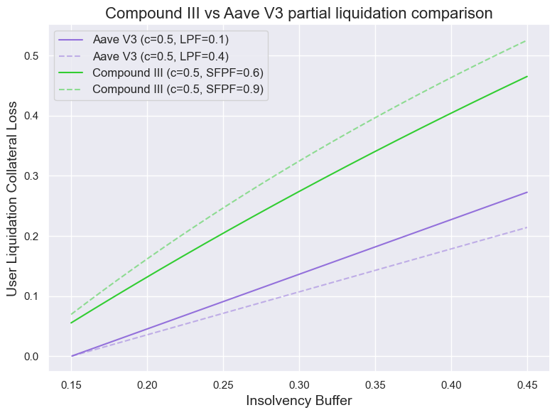
The effects are more pronounced here since charging more per liquidation improves the IB more than charging less per liquidation but increasing the LP. This is because protocol fees directly go towards the IB whereas the LP goes towards the liquidator.
Overall, partial liquidations don’t seem to provide a substantial competitive improvement given that Compound III still mostly lags Aave V3 with the change.
Differential impact of partial liquidations
This aim here is to provide a quantitative comparison for partial liquidations vs full liquidations.
New comparison model
The IB framework works well for comparing Aave and Compound, but it is less helpful when comparing partial liquidations to full liquidations. It tends to imply that partial liquidations are always better since they appear to pay less for the same amount of risk reduction.
In fact, the highest possible IB corresponds to no liquidation at all since the protocol avoids paying out any collateral via liquidation penalties. But this doesn’t account for the value of actually reducing risk. A full absorption has the useful property that once the liquidation is executed, the protocol no longer bears collateral price risk. By contrast, avoiding liquidation entirely might preserve more buffer up to the point of insolvency but leaves the protocol fully exposed if the price keeps falling.
In essence, partial liquidations pay less in exchange for time. But that time often works against the protocol since price is typically moving unfavorably in those moments. Full liquidations are more valuable when the price is dropping block by block.
To capture this tradeoff, define the block insolvency buffer (BIB) as the maximum percentage the collateral price can fall relative to the debt per block between absorption and sale before Compound III takes a loss.
Deriving a relation between BIB and close factor c will give some intuition on the risk incurred from partial liquidations.
Model derivation
Define d \in [0, 1] as the % the price of the collateral drops each block and define k_i as the block number where the i th partial liquidation occurs starting with k_1 = 1. Assume that the absorbed collateral is sold entirely in the following block and that gas is negligible relative to the liquidation proceeds so this process can go on indefinitely.
In every liquidation 1-c of the collateral remains in the account and the value of the collateral is discounted by 1-d every block so by the i th liquidation the amount of collateral remaining is given by C(1-c)^{i-1}(1-d)^{k_i}. The liquidation involves selling c of this remaining collateral at a discount of 1-LP\cdot SFPF so the total value of the collateral as a result of the i th liquidation is given by cC(1-LP\cdot SFPF)(1-c)^{(i-1)}(1-d)^{k_i}.
The amount of base asset credited to the borrower during the i th absorption is 1-LP multiplied by the value of the collateral absorbed which is given by C(1-c)^{i-1}(1-d)^{k_i-1} Note that this is similar to the expression for collateral remaining by the i th liquidation but the conversion to base asset occurs at absorption and before the liquidation completes in the following block, hence the difference by a factor of 1-d. Since c of this collateral is absorbed the total amount credited during the i th absorption is given by cC(1-LP)(1-c)^{i-1}(1-d)^{k_i-1}.
Putting this altogether the net payout for the protocol A is given by
A(d) = cC(1-LP \cdot SFPF)\sum_{i=1}^{\infty}{(1-c)^{i-1} (1-d)^{k_i}}
- \max\bigg(D, cC(1-LP)\sum_{i=1}^{\infty}{(1-c)^{i-1}(1-d)^{k_1-1}}\bigg)
Consider the special case where partial liquidations occur every block so k_i = i \hspace{2mm} \forall i \in \mathbb{Z}^{+} (as an example this would happen if D = C(1-LP)) and define the net payout in this case as \widehat{A} so
\widehat{A}(d) = cC(1-LP \cdot SFPF)(1-d)\sum_{i=1}^{\infty}{(1-c)^{i-1} (1-d)^{i-1}}
- \max\bigg(D, cC(1-LP)\sum_{i=1}^{\infty}{(1-c)^{i-1}(1-d)^{i-1}}\bigg)
so then simplifying the geometric series we get
{\widehat{A}(d)} = \displaystyle\frac{cC(1-LP\cdot SFPF)(1-d)}{1-(1-c)(1-d)} - \max\bigg(D, \frac{cC(1-LP)}{1 - (1-c)(1-d)}\bigg)
Let \widehat{d} be the solution to \widehat{A}(d) = 0. Substituting D = C \cdot LF we obtain
\widehat{d} = \begin{cases} 1 - \displaystyle\frac{LF}{c(1-LP\cdot SFPF) + LF (1-c)} & \text{if } \widehat{d} > \displaystyle\frac{c(1-LP-LF)}{(1-c)LF} \\[2ex] 1 - \displaystyle\frac{1-LP}{1-LP \cdot SFPF} & \text{if } \widehat{d} \leq \displaystyle\frac{c(1-LP-LF)}{(1-c)LF} \end{cases}
which further simplifies to
\widehat{d} = \begin{cases} 1 - \displaystyle\frac{LF}{c(1-LP\cdot SFPF) + LF (1-c)} & \text{if } c < \widehat{c} \\[2ex] 1 - \displaystyle\frac{1-LP}{1-LP \cdot SFPF} & \text{if } c \geq \widehat{c} \end{cases}
where
\widehat{c} = \displaystyle\frac{LF \cdot LP(1-SFPF)}{(1-LP)(1-LP \cdot SFPF -LF)}
Note that \widehat{c} can be rewritten as \displaystyle\frac{LF}{1-LP} \cdot \frac{LP - LP \cdot SFPF}{1-LF - LP \cdot SFPF} which safisfies c \in [0, 1] since SFPF \in [0, 1] and LF + LP \leq 1 by definition.
Proof that \widehat{A} \geq A
Let’s define
\widehat{F} = cC(1-LP \cdot SFPF)\displaystyle\sum_{i=1}^{\infty}{(1-c)^{i-1} (1-d)^i}
F = cC(1-LP \cdot SFPF)\displaystyle\sum_{i=1}^{\infty}{(1-c)^{i-1} (1-d)^{k_i}}
\widehat{G} = cC(1-LP)\displaystyle\sum_{i=1}^{\infty}{(1-c)^{i-1}(1-d)^{i-1}}
G = cC(1-LP)\displaystyle\sum_{i=1}^{\infty}{(1-c)^{i-1}(1-d)^{k_1-1}}
Then \widehat{A}(d) = \widehat{F} - \max(D, \widehat{G}) and A(d) = F - \max(D, G)
Note that \widehat{F} \geq F since every term is both expressions is nonnegative with c, d, LP, SFPF all in [0, 1] and C \geq 0 but the terms in F are a subset of the terms in \widehat{F}
Similar reasoning applies to show that \widehat{G} \geq G since LP \in [0, 1] as well
So this gives 3 cases
\textbf{Case 1:} \hspace{1mm} G \geq D
Then \widehat{A}(d) - A(d) = (\widehat{F} - F) - (\widehat{G} - G)
This difference can be expressed as the following series
\bigg(cC(1-LP \cdot SFPF)(1-d) - cC(1-LP) \bigg) \displaystyle\sum_{\begin{subarray}{c} j=2 \\ j \notin \{k_i\}_{i\in \mathbb{Z}^{+}} \end{subarray}}^{\infty}{(1-c)^{j-1} (1-d)^{j-1}}
We note that the expression cC(1-LP \cdot SFPF)(1-d) - cC(1-LP) is always nonnegative if d \leq 1 - \displaystyle\frac{1 - LP}{1 - LP \cdot SFPF} = IB_{\max} which holds since the single block IB upper bounds the multiple block BIB.
\textbf{Case 2:} \hspace{1mm} \widehat{G} \leq D
Then \widehat{A}(d) - A(d) = \widehat{F} - F \geq 0
\textbf{Case 3:} \hspace{1mm} \widehat{G} \geq D \geq G
Then \widehat{A}(d) - A(d) = (\widehat{F} - F) - (\widehat{G} - D) = (\widehat{F} - F) - (\widehat{G} - G) + (D - G) \geq 0 by the same reasoning as Case 1
so \widehat{A}(d) \geq A(d)
Why did we do all this math
Finding an explicit analytic solution to the general model is hard. The special case is easy to solve and provides a clear bound for the optimal solution.
A is decreasing in d since larger collateral drops per block is worse for the protocol’s net payout so if d^{*} is the solution for A(d) = 0 then A(\widehat{d}) \leq \widehat{A}(\widehat{d}) = 0 so \widehat{d} \geq d^\star.
It follows that if c^{*} is the solution for A(d) = 0 then c^{*} \geq \widehat{c} since a smaller insolvency buffer means the protocol should close out debt more aggressively.
Now there is a formulaic lower bound for what the close factor should be set to.
Analysis
Using the risk parameters for WBTC and plotting our upwards biased estimator of BIB against a numerical approximation for the true BIB gives

The dotted curve shows the BIB in the idealized case where partial liquidations happen every block. Once the cumulative value of absorptions exceeds the original debt, the BIB converges to the IB. In this case, a partial liquidation offers the same level of insolvency protection as a full liquidation but at a lower cost to the user’s collateral.
In practice, liquidation delays are unavoidable, so the solid curve illustrates the more realistic relationship between BIB and c. The gap between the two curves reflects the risk introduced by those delays. In this example, the BIB is concave, suggesting that setting the close factor between 0.4 and 0.6 may strike a reasonable balance between insolvency protection and user collateral costs, though this should be calibrated per asset.
If properly tuned, partial liquidations can offer similar risk protections as full liquidations for a reduced cost.
Suggested solutions
Since the competitive impact of this change is unclear but the impact of the change in a vacuum is positive, the solution should orient towards simplicity and low risk and costs.
Because of Compound III’s design, partial liquidations face some added wrinkles. Typically the liquidator repays a proportion of debt and selects collateral to repurchase. On Compound, the liquidator needs to absorb the collateral first before repaying debt in the subsequent collateral sale. This opens up some design choices around which collaterals and how much of each should be eligible to be absorbed (noting that there is no function to unabsorb), whether this should be chosen by the liquidator etc.
Using @torrey’s earlier suggestion of using a close factor for the entire account greatly simplifies this. This leads to the following solutions
Partial absorptions through close factor
The isLiquidatable function can remain unchanged. Depending on the change surface the AssetInfo struct could be expanded to take a close factor per asset. If this is onerous then setting to a default of 0.5 as a new comet parameter in the Configurator seems reasonable. The absorbInternal function should be updated to account for the close factor.
Partial absorptions through target health factor
Another possibility is to have a maximum health factor like Euler V1 set to 1.25 here. Then modify absorbInternal to accept an extra parameter which determines the proportion of the account to be absorbed and have a health factor check that reverts if it exceeds the maximum HF. The corresponding close factor can be explicitly derived as follows
Formula derivation
Suppose an account has N collateral assets where C_i is the value of i th collateral and let D denote the value of the debt in the base asset. Let LF_i and LP_i denote the liquidation factor and liquidation penalty of the i th collateral and let T^{*} denote the target health factor
Define the health factor
Now following partial liquidation over a proportion c of the account, the new health factor would be
Equating this to the target health factor T^{*} and solving to get the optimal close factor c^{*} gives
Note that D \leq \displaystyle\sum_{i=1}^{N}{C_i(1-LP_i)} or else c^{*} > 1. Recall that LF_{i_{\text{max}}} = 1 - LP_i. This corresponds to the case where if the debt exceeds this amount \displaystyle\sum_{i=1}^{N}{C_iLF_{i_{\text{max}}})}, the liquidation actually makes the health factor worse.
Following from that bound, if both the numerator and denominator of the expression were negative then c^{*} \geq 1 so it follows that T^{*}D \geq \displaystyle \sum_{i=1}^{N}{C_i LF_i} or else c^{*} < 0. Rearranging this corresponds to T^{*} \geq \frac{\displaystyle\sum_{i=1}^{N}C_iLF_i}{D} = HF so the target health factor must be at least the current health factor
Empirical analysis
One way to determine what value to set the target health factor to be is to look at important historical liquidations. Averaging all liquidations in Compound III larger than 10M which accounts for roughly 35% of total liquidation volume gives the following

From this, a target health factor of 1.05 seems reasonable.
Really excited to see liquidation improvements on Compound. Hope this was a helpful overview. Happy to discuss further on the next community call and continue our collaboration!