[RFC] Partial Liquidations

[woof]

Intro

Liquidations are bad for both protocol and users:

• Liquidated positions don’t accrue interest (fees).
• Borrowers lose collateral.

Liquidations are inevitable, but damage can be decreased by liquidating a part of the borrowing position, instead of absorbing the full collateral value.

Partial liquidations are a key component in increasing the Collateral Factor (Loan-to-Value).

This post describes how partial liquidations can be implemented within the Compound v3 infrastructure.

Motivation

The current Compound Comet model is based on the evaluation of the health factor of the user’s account based on the collateralization factors for each collateral asset.

Note: To lay the basis, let’s start from the loan-to-value (LTV) definition, which characterizes the user’s position in the protocol. Based on the agreed notion (in both traditional sources, web3 resources, and Compound itself), LTV is always defined as the ratio of debt / collateral value. And, transitionally, the same applies to collateral factors and liquidation factors, represented in numbers below 100% (below 1). Therefore, we will keep the same notion and represent Health Factor (HF) as a ratio of debt / collateral value (scaled by collateral factors). So, if HF is less than 1, then the account’s collateral (scaled) covers the debt; if the collateral factor is more than 1, then the debt exceeds the collateral value. And it is in congruence with the loan-to-value ratio, as the health factor is its direct descendant.

HF (Health Factor) is a ratio between debt and collateral value, factored by the collateral factor:

1. HF = \frac{ (\text{principal} + \text{interest}) \times \text{base asset price} }{ \sum_{i}^{n} \left( \text{collateral balance}_i \times \text{collateral price}_i \times \text{collateral factor}_i \right) }

Once HF increases above 1, the user is not able to increase the loan. However, a user’s liquidation occurs only after the user falls under the liquidation threshold.

LF (liquidation factor) is a ratio between the user’s debt and the collateral value, factored by the collateral liquidation factor:

2. LF = \frac{ (\text{principal} + \text{interest}) \times \text{base asset price} }{ \sum_{i}^{n} \left( \text{collateral balance}_i \times \text{collateral price}_i \times \text{collateral liquidation factor}_i \right) }

The protocol keeps HF >= LF (as collateral factor < collateral liquidation factor)

Once LF grows above 1, the user will be liquidated. And in this case, the protocol seizes the full amount of collateral, though it leaves a difference after the debt coverage with the discounted value of the collateral.

Such an approach leads to 2 issues:

1. Users (in general) lose all of their collateral.

While it is consistent with the protocol’s mechanics, which protects it from bad debts, it creates a downside for a user willing to pay the interest but short on time to collect additional collateral. Thus, such a user (with the health factor pushed to be right above the liquidation threshold) who could bring more profit in perspective by paying interest, will lose the position. Another factor to take into consideration - if the user has more collateral value (scaled down by penalty) than the debt, then the difference between collateral value and debt is returned to the user as principal balance in the base asset. Thus, the user gets a “virtual swap” of collaterals to the base asset, which (after the withdrawal) will decrease the overall supply - and so it acts as a factor that contaminates the growth of the reserves.

2. Liquidators should cover the whole debt position.

By default, it is assumed that the protocol absorbs the position below the liquidation threshold. In that case, the protocol closes the user’s debt and seizes collateral with a penalty into the reserves. So there exists a “virtual swap” where the protocol “swaps” debt denominated in base asset to collateral denominated in other assets. So, the base asset supply is increased by a value of closed debt, but it is actually presented as a sum of collaterals instead of the appropriate amount in the underlying. And since the protocol should protect lenders who provided the liquidity, it should bring the same base asset amount back to the pool. Thus, the protocol sells collaterals back to liquidators at a discounted price, but this is still higher than the liquidation factor. So, after 2 actions (debt absorption and collateral sell), the protocol gets back the necessary base asset amount. However, this operation assumes that liquidators will have enough base asset amount in the first place, and that assumption limits the number of liquidators willing to participate in the liquidation process and limits the retention of the base asset liquidity back to the protocol.

The main motivation under the partial liquidation is:

• To decrease the average amount of base assets, the liquidators should have to participate in the liquidation process;
• Decrease the number of cases when the user loses the whole position and increase the lifetime of the position, maximizing the amount of potential interest.

And vice versa, the partial liquidation itself brings additional motivation for the ecosystem participants:

• It gives a mechanism that will help users keep the account’s health for a longer period.
• It encourages liquidators with low- and medium-sized portfolios to participate in liquidations;
• Together, both mechanisms work on keeping healthy accounts and avoiding bad debts, as they operate with smaller amounts.
• Additionally, partial liquidation works on the prevention of cascade liquidations of monolithic liquidity, working on the health of the whole system

Basis

Before the solution development, we define the basis for it - as the partial liquidation should not disrupt existing protocol mechanics. Therefore, we base the solution on the following principles:

1. The solution should keep a fair competition between liquidators.
2. The solution should not disrupt an existing mechanism for liquidators.
3. The solution should not increase the amount of bad debt in the system - vice versa, it should encourage ecosystem participants to avoid bad debt.
4. The solution should, at maximum scale, re-use the existing liquidation mechanics. We need to avoid building a new infrastructure or implementing breaking changes into the existing liquidation process.
5. The solution should not discourage liquidators from full liquidation if they want such; however, partial liquidation should become a preferable option.
6. The solution should keep minimal changes in the protocol’s codebase, ideally, with no modifications in existing functions, but only with the implementation of new ones.

Solution

The solution can be expressed in a single sentence: give liquidators a debt amount they should cover for a user, to bring the user’s HF back above the liquidation threshold.

If expressed in a formula (using HF and LF formulas from 1. and 2.):

3. \text{If } (LF > 1), \text{ then find such } \Delta \text{debt so that } LF < 1

However, having LF as a target is inconvenient, as once we bring it back to 1, the accrued interest will exceed the LF again. Instead, we’ll use the fact that when LF = 1 it corresponds to a certain value of the health factor, which we can name LHF (liquidation health factor).

Let LHF (liquidation health factor) correspond to HF when LF = 1.

Example:

• collateral factor = 0.825
• collateral liquidation factor = 0.85
• Collateral price = 2000$
• Collateral balance = 1

It gives:

• HF = 1 with maximum debt of 1650$ (collateral balance * price * collateral factor)
• LF = 1 with debt exceeding 1700$ (collatearal balance * price * liquidation factor)
• When LF = 1, the appropriate health factor equals:
  LHF = debt / (collateral balance * price * collateral factor) = 1700$ / 1650$ = 1.03

So, now we can define the target HF (or min HF) to achieve, to keep account above the liquidation threshold:

4. \text{target } HF < LHF

Where LHF is a health factor when LF = 1.

Now we can reformulate the solution as:

5. \text{If user's } LF \geq 1, \text{ then find such } \Delta \text{debt so that } HF = \text{target } HF

Note: In Comet, all debt balance calculations are performed in terms of principal scaled by the borrow index, to represent (principal + interest). So we can safely refer to debt as (principal + interest) to simplify the equation. Also, let’s define debt as (debt * base asset price) to avoid extra multiplier in notation. Additionally let’s substitute collateral value calculations with collateral value = (collateral balance * collateral price) - again to avoid extra price multiplier (since it is never used without connection to the balance)

Expressed in formula (based on formulas (1) and (2):

6. LF = \frac{ \text{debt} }{ \sum_{i}^{n} \left( \text{collateral value}_i \times \text{collateral liquidation factor}_i \right) }
7. \text{target } HF = \frac{ \text{debt} - \Delta \text{debt} }{ \sum_{i}^{n} \left( (\text{collateral value}_i - \Delta \text{collateral value}_i) \times \text{collateral liquidation factor}_i \right) }

Compound siezes the collateral from the user with a penalty. So:

8. \text{debt} \leq \sum_i \left( \text{collateral value}_i \times \text{liquidation penalty}_i \right)

We can safely use the border case of equality - when the penalized collateral fully covers the debt and equals it. In case the debt exceeds the available collateral, the difference will just be added to the user’s balance, in the same way it works during the absorption.

9. \text{debt} = \sum_i \left( \text{collateral value}_i \times \text{liquidation penalty}_i \right)

It allows us to express the difference the liquidator should pay as:

10. \Delta \text{debt} = \sum_i \left( \Delta \text{collateral value}_i \times \text{liquidation penalty}_i \right)

And now the task is to find the 𝚫collateral value to substitute it and get 𝚫debt the liquidator should pay.

Using equation (7):

11. \text{target } HF = \frac{ \text{debt} - \sum_{i}^{i} \left( \Delta \text{collateral value}_i \times \text{liquidation penalty}_i \right) }{ \sum_{i}^{n} \left( \left( \text{collateral value}_i - \Delta \text{collateral value}_i \right) \times \text{collateral factor}_i \right) }

This is the place to apply a rule: the liquidator should set the collateral to seize and the order of collaterals to get and use one collateral at a time. We need to apply such a rule to simplify the equation:

• we cannot assume that the liquidation penalty, liquidation factor and collateral factor are the same for all collaterals;
• We cannot limit partial liquidations to single-colateral loans.
• We cannot work with equations with multiple unknowns
• So we need to split it into a system of consecutive equations.

12. \text{target } HF = \frac{ \text{debt} - \Delta \text{collateral value} \times \text{liquidation penalty} }{ \left( \text{collateral value} - \Delta \text{collateral value} \right) \times \text{collateral factor} }

Now, by simplifying expression (12) we can express delta collateral:

13. \Delta \text{collateral value} = \frac{ \text{debt} - \text{collateral value} \times \text{collateral factor} \times \text{target } HF }{ \text{liquidation penalty} - \text{collateral factor} \times \text{target } HF }

Returning to the 𝚫debt equation (10), we can give to the liquidator the amount of base asset the liquidator should pay to seize a certain collateral to bring the user back above the liquidation threshold.

Edge-cases

The solution also covers the row of exceptions and edge cases:

Q: What if the user does not have enough collateral of this type (equation (12))?
A: The rule states to use one collateral at a time and to define an order of collaterals to seize. So, if the calculation shows 𝚫collateral value that exceeds the collateral balance of the user - just use the full balance, and go to the next collateral to calculate its 𝚫 - up until there are enough collaterals:

14. \text{target } HF = \frac{ \text{debt} - \left( \text{collateral value}_1 \cdot \text{liquidation penalty}_1 + \Delta \text{collateral value}_2 \cdot \text{liquidation penalty}_2 \right) }{ \left( \text{collateral value} - \text{collateral value}_1 \cdot \text{collateral factor}_1 - \Delta \text{collateral value}_2 \cdot \text{collateral factor}_2 \right) }

• And calculation repeats with the updated debt value and new collateral
• The cycle for calculation will be similar to the ones used in isBorrowCollateralized() and isLiquidatable() functions

Q: What if the debt from the start falls under the condition of the bad debt (equation (8) is disrupted) ?
A: Have a check on bad debt before any partial liquidation, similar to the collateral or liquidation checks in withdraw() and absorb() functions. And then follow the existing liquidation flow.

Q: Is this partial liquidation consistent with the full liquidation mechanics, which are already implemented?
A: In short - yes.
The maximum value that can be liquidated is debt itself.
The maximum value the user can lose is:

• The whole collateral amount in case of bad debt;
• Exactly all collateral if 𝚺(collateral value_i * liquidation penalty_i) = debt (if penalized collateral covers debt exactly);
• 𝚺(collateral value_i) - (𝚺(collateral value_i * liquidation penalty_i) - debt) otherwise (in case if penalized collateral covers more than current debt)

Debt to repay in partial liquidation is calculated exactly based on penalized collateral, thus neither user can lose more than that during full liquidation, nor can the liquidator acquire more assets than that during full liquidation.

Q: The equations are based on the equality of debt calculation and penalized collateral value. What if the user falls under the liquidation threshold, but still has enough collateral to cover the debt with a penalty?
A: Assumption is based on the fact that penalized collateral will be seized anyway in case of full liquidation, thus it’s safe to calculate it this way from the start. During partial liquidation, the user cannot lose more collateral than necessary to cover the debt. Thus, the other difference will remain.

Q: What is the minimal amount of debt to be repaid via the partial liquidation flow?
A: The 𝚫debt calculated is actually the smallest amount of debt to repay to bring the account back to the target HF. So, it depends on the target HF set for a pool. And, to avoid micro payments, the functionality will be enforced to have the user’s LF <= 1 at the end of the function.

However, additional restrictions can be implemented to bound the partial liquidation to a % of a user’s debt to cover (e.g., not less than 20% of the debt with fulfillment of the equations above).

Q: How to calculate the target HF (target health factor) ?
A: Based on the definition, the next should be applicable:

HF <= target HF <= LHF

So, it can have a respective storefront coefficient, as
Target HF = x% of LHF

For example:

• With the example used in the LHF we have LHF = 1,03
• The storefront coefficient can be set as: x = 98%
• Target HF = x% of LHF = 98% of LHF = 1,0094

So it can be easily computed for each user respectively as:

15. LHF = \frac{ \sum_{i}^{n} \left( \text{collateral value}_i \cdot \text{collateral liquidation factor}_i \right) }{ \sum_{i}^{n} \left( \text{collateral value}_i \cdot \text{collateral factor}_i \right) }

Target HF = x% * LHF

Q: How to encourage liquidators to perform partial liquidations instead of full liquidations?
A: There are several ideas that require feedback:

• (requires new parameter for assets): Allow partial liquidation to start earlier than full liquidation - implement a sub-liquidation factor (lower than the liquidation factor), which will be used to check if a user is eligible for the partial liquidation (partial liquidations will start on a lower HF than full liquidation).
• (requires new parameter for assets): Increase the discount on sold collateral during the partial liquidation operation compared with the full liquidation (liquidators get more collateral cumulatively);
• (requires new parameter for assets): Increase the penalty on seized collateral compared with the full liquidation (so more collateral is seized in general compared with full liquidation);
• Add more liquidation points during the partial liquidation (to influence further rewards distribution).
• Boost partial liquidation with separate rewards.
• Add a bonding curve or a linear decrease in the discount for the liquidation, from minimal to the full (so that immediate partial liquidation will bring more cumulative profit than the full liquidation of the same amount).

For now, we prefer to have the combination of “early start” for partial liquidations together with the linear growth of liquidation discount:

• Introduce a new threshold for assets - PLF, partial liquidation factor (collateral factor <= PLF <= liquidation factor). It will define a respective PLHF (partial liquidation health factor). Thus, HF <= PLHF <= LHF <= bad debt health factor
• That gives an interval for the debt to fall (from PLHF to LHF) and be eligible for partial liquidation
• Bound the liquidator’s discount to the Target HF / actual HF value, to have an increased discount for early partial liquidations
• Once LHF is achieved, the liquidator’s discount is the same for full liquidation and partial liquidation, and it is up to a liquidator to decide.
• Note: idea is equivalent to having a liquidation penalty linearly dependent on the Target HF / actual HF ratio. Thus, liquidation penalty is another parameter to work with - with the currently set penalty (in assetInfo.liquidationFactor) staying as the final lowest penalty to achieve.

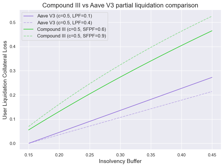
Modeling results

Partial liquidation modeling

Implementation

Implement new storage:

• Global parameter to represent the storefront coefficient for the decrease of LHF to HF (for Target HF calculation).

Implement new functions:
1. collateralValues()

• The utility function that gets collateral values and caches them (to avoid frequent oracle calls)
• Structure is similar to isLiqidatable() and coisBorrowCollateralized()
• Returns array of collateral values

2. isBadDebt()

• Structure is similar to isLiqidatable() and coisBorrowCollateralized()
• Uses cached collateral values from collateralValues()
• Checks the factorized sum based on assetInfo.liquidationFactor

3. Additional viewers:

• targetHF() - function to calculate the minimal health factor account needed to set account above the liquidation threshold
• minimalDebt() - function to return the minimal debt value to repay to set up over the liquidation threshold (based on equations (10) and (13))
• collateralForDebt() - helper viewer based on the equation (13) to show how much collateral can be seized for a partially closed debt.

4. absorbPartial()

• Gets an array of collaterals to seize and account to liquidate
• Gets amount of debt the liquidator is willing to repay
• Checks if the user has bad debt
• Uses cached collateral values from collateralValues()
• Calculates LHF for the user
• Calculates Target HF for the user
• Calculates delta collateral based on equations (13) and (14) - cycle is similar to isLiqidatable() and coisBorrowCollateralized() (note - all prices are cached at the beginning of the function, so no additional storage reads are present)
• Calculates the minimal delta debt to cover
• Expect not less debt to be covered than delta debt.
• Updates the user’s principal, total supply and total borrow values
• enforces the rule that the health factor after the absorption should be <= target HF

In general, the function’s structure is similar to the absorb() function

And so the same is the next step for the liquidator - call buyCollateral() function to return the base asset into the pool. This call can be enforced in the same function (the result depends on the final gas testing).

5. Changes on an incentivisation of partial liquidations depend on the final decision on the form of liquidation. Though the preferred approach includes:

• Adding a new factor for assets (recorded in assetInfo) - PLHF;
• Adding new viewers similar to isLiquidatable() : isPartiallyLiquidatable()
• Viewer to calculate starting discount and final discount based on linear model and with existing values (assetInfo,liquidationFactor and storefrontPriceFactor) as input values
• Integration with the new partialAbsorb() function and buyColalteral() function.

Next steps

• Community Discussion
• Technical Scoping
• Snapshot Vote
• Implementation

[torrey]

@woof

Thus, the user gets a “virtual swap” of collaterals to the base asset, which (after the withdrawal) will decrease the overall supply - and so it acts as a factor that contaminates the growth of the reserves.

I’m not sure I agree with this statement. In the past we’ve seen liquidations actually contribute to massive growth of reserves of a market because of the corresponding sale of the collateral back to users who wish to purchase it at a discount. The sale of the collateral absorbed from the liquidation is what contributes to reserve growth as well.

@woof

Liquidators should cover the whole debt position.

This section is not quite true either. The protocol actually is what assumes the whole debt position (in the form of reducing reserves). The protocol then recovers its reserves by selling the seized collateral at a discount to anyone who wants to buy it. The selling of the seized collateral is what then contributes to reserves once more to fill in the gap made by taking ownership of the absorbed debt. No liquidator needs to cover the whole of anything, rather buyers of the seized collateral only need to worry about how much of whatever seized collateral they want to purchase from the protocol collateral reserves. It is for this case that reserves are even allowed to go negative during an absorb while the seized collateral is waiting to be bought.

---

What if we instead start with adjusting the absorb() function to some percentage of a user’s position? (This was tough to identify in v2 what this percentage level should be depending on various states of prices in the market). We could come up with a model that says at minimum x% of a user’s total debt (vs 100% currently) is able to be absorbed by the protocol at all times which is a bit safer for the user to defend their position while also ensuring a position is also attractive for users who wish to trigger the absorption. I do not think that only allowing the current underwater debt amount to be absorbed is the correct approach, especially in severe conditions but I would defer risk on this to Guantlet. Adjusting the absorb() is probably the quickest change to implement as well with minimal changes to the whole liquidation system.

If the protocol is responsible for absorbing a position, the protocol can also attempt to seize all collateral fairly vs a case where some liquidators may only want specific collateral assets to seize if the protocol leaves the decision up to a liquidator. This is a far better experience for the borrower. I do still think allowing anyone to purchase seized assets from the protocol itself is a great experience for anyone who wants to purchase assets at a discount, though traditional liquidators are the ones here who are probably the quickest. Allowing liquidators to choose which collateral they want is likely pretty bad for borrowers as only the highest collateral factor assets are likely to be taken first meaning the borrower will lose those assets first in a falling market environment.

There should be discussion however on Liquidator Points, as that is what is accrued to users who liquidate by calling absorb() which absorbs bad debt positions into the protocol. Currently Liquidator Points are tracked but nothing is currently done with those points.

To give a little context, the v2 Compound Protocol does support partial liquidations, however we designed the separate Liquidation Factor (LF) in v3 in order to better protect user’s positions by giving them some extra buffer to defend their positions beyond just the Collateral Factor. Additionally, for v3 we made the decision to absorb an entire debt position during a liquidation vs reading a Close Factor that existed in v2 because we noticed that there were lots of positions in v2 that could never be closed resulting in just stale assets that will likely just sit there forever. I think we can find a better middle ground here.

[Midvel]

Hey, thank you for the detailed feedback! I’m Pavlo, a Solutions Architect at WOOF! who worked on the solution and its reasoning. Let me answer the raised statements.

1. The core question is - what exactly should be that percentage x% of a user’s debt that the protocol will allow to repay? The point is - it should be enough to bring the user above the liquidation threshold and it should be enough to not trigger immediate liquidation again. The post above already provides an approach to resolving minimal debt to achieve a target health factor. So, keeping all calculations, it may serve as a minimal target, AND now we can add a percentage of the repaid debt upon it (thus increasing the repaid amount but still keeping it partial).
2. The next logical query: why should we still have the target HF and minimal debt calculation instead of just having a fixed % to repay? First of all, it is an orienteer for liquidators on the amount of debt enough to bring the user back into the healthy account, and secondly - it works for the flexibility, as seizing fixed % of debt in any situation is still in some sense analogous to a full liquidation but with less collateral seized, and it still limits small- and min-sized liquidators.
3. However, in general - yes, %x of the debt can be implemented, but it still will require most of the checks described in the document. So I’d still advise to have all underground calculations - but they can be covered with a nice % parameter for convenience. Though, in some way, it will not be a partial liquidation in its pure definition, but a fixed % liquidation. It is a better condition for a user than a full liquidation, but still harsh enough.
4. As for keeping collateral purchase and absorption separate. That is fair, though an approach to unite these operations for partial liquidations was offered to allow liquidators to choose the collateral to seize and purchase it immediately + to have adjustments for the liquidator’s discount based on partial liquidations. Without it, the incentive to push the partial liquidation over the full liquidation will be only in a specific collateral choice and maybe the implementation of a higher penalty (as the liquidator should be able to have some incentive). So, it is still an option to consider, as dividing these functions is convenient for the protocol itself (in case the protocol triggers the liquidation), but as for the liquidator, it will be convenient to have the atomic seizing of the collateral. So, the functionality can be left intact for protocol-based liquidations (with a registry of protocol’s liquidators) and can be united for a partial liquidation flow. On the implementation level it can be just a flag in the absorb() function indicating if the liquidator is willing to purchase collateral immediately.
5. As for the liquidator points as incentives (instead of playing around penalty or discount) - it is a point of discussion, as indeed it is a whole functionality unused but which can be utilized for incentives - implementation can contain bonus points for the partial liquidations.
6. As for LF implementation discussion - indeed, and LF is the exact border we are playing around with a partial liquidation as well.
7. As for positions that are never closed - that is a completely different question, probably for working with position maturity. E.g., mature positions cannot be eligible for partial liquidations, only for full liquidations. That will solve the problem of stale liquidity, still allowing the partial liquidation. However, with current absorption flow it seems not to be a problem - as even with partial liquidations, there is a threshold after which the position (decreased during several partial liquidations) will be closed completely with no stale liquidity in the end.

So, in short:

• %x over debt can still be implemented with the target HF and minimal debt under it - though we still think that higher flexibility will work better for liquidators as it will engage new audience
• split between absorption / collateral purchase - it can be split for the protocol-triggered liquidations, though it is still advised to be united for partial liquidations (implemented as a simple flag in a absorb() function)
• as for liquidator points - that is a good incentive mechanism which is currently unused. We can offer e.g. a reversed bonding curve to connect liquidator points to a percentage of debt closed. Though in that case, an additional rewards mechanism should be developed - e.g., a higher discount during a collateral purchase based on liquidator’s points accumulated (thus it will trigger slow burning of liquidator points without the need to unite operations of absorption and purchase)
• to avoid stale liquidity, an additional maturity factor can be introduced, after which only full liquidations are allowed, though again - it seems not to be a problem, as position will be closed anyway after a certain threshold/number of partial liquidations

[woof]

Community Feedback Integration
We’ve received valuable community input regarding liquidation mechanisms and implementation approaches. As part of our implementation process, we will explore additional configuration options that could provide liquidators with enhanced flexibility and improved user experience.
These considerations may include investigating:

• Percentage-based liquidation parameters for simplified liquidator interaction
• Enhanced liquidator points utilization for partial liquidation incentive mechanisms
• Flexible absorption and collateral purchase workflows to optimize liquidator experience
• Fair collateral distribution approaches to ensure equitable access across participant types
• Additional configuration parameters for diverse liquidation strategies and risk management

Any such enhancements would be designed to complement the existing target health factor methodology while maintaining the core safety mechanisms and mathematical foundations outlined above. We remain committed to iterating on the implementation based on community needs and real-world usage patterns, ensuring the final solution serves the broadest range of ecosystem participants effectively.

[jbass-oz]

Partial Liquidations RFC - OpenZeppelin Response

Introduction The following response has been prepared after a Request For Comment (RFC) on Partial Liquidations. It is not a critique of partial liquidations as a concept, but is instead intended to highlight areas of the Partial Liquidations [RFC] which may need further elaboration or refinement. The intention being to raise concerns as early as possible before development starts. While the RFC frames liquidations as bad for the protocol and users, it should be noted that liquidations form a c…

[woof]

Thanks to OpenZeppelin for valuable feedback and the support of the partial liquidation initiative. It is highly appreciated when the security provider supports the ecosystem enhancement initiatives and engages in active discussions.

First of all, we agree that liquidations are a natural mechanism designed to maintain the health of the protocol and to serve as an extension of the ecosystem, introducing independent participants. The thoughts in RFC are targeted at the full over-liquidation, which creates a set of risks already described in the RFC and with some key points which were noted by OpenZeppelin during the audit of the Compound (as an over-liquidation and as a point of additional monitoring).

As for the points raised in the report.

1. Partial Liquidations and Target Reserves

The role of the targetReserves in the Comet was already discussed during the Compound III audit, as it was noticed that the chosen strategy of holding reserves may not be optimal. However, the role of target reserves is not discussed within this particular RFC, as it has no intention of changing that logic and has no impact on the fulfillment of targetReserves:

• The RFC aims to keep the invariant of closing off collateral purchases after the targetReserves are reached;
• Operations unification (absorb+purchase) does not mean the violation of the target reserves, as it is a matter of implementation. Thus, the RFC poses no intent on changing this logic, but working around the user interface only.
• Additionally, based on the received feedback, the unification is not mandatory, but rather optional, solely for the convenience of the liquidator.

Thus, thank you for highlighting the point, but the concern is primarily related to the specific implementation rather than the solution itself. The team will keep this in mind and add it as an additional invariant to be maintained during solution testing.

2. Selective Collateral Seizure

The point describes the possibility of meeting the grief risk, connected with the seizure of a particular “strong” collateral. First of all we need to notice, that the current implementation of the liquidation possesses a part of such a risk: the order of collaterals in the Comet is mostly arbitrary, thus there are situations when the “strong” collateral is placed first, and during the full liquidation it is the first to be seized. Thus, even now, there exist situations when the user will end up with a “weaker” portfolio and will not be able to enter the debt position again. And vice versa - based on the order of collaterals, the Comet may end up with higher reserves of “weaker” collaterals seized during the liquidations. Thus, in general, such a risk (while having low likelihood) is present even now.

However, the feedback contains a valuable point that indeed, the allowance of collateral choice may impact the behavior of liquidators. Though during the RFC preparation, this risk was analyzed, and the solution is based on certain points:

• From the Comet point of view, all collaterals are equal, as there is no ordering and ranking of collaterals to point to particular ones.
• All collaterals are limited by their respective caps; thus, even if some collateral is seized more frequently, it will create a natural flow of its supply back, as other collaterals are limited in their caps.
• Even if a “stronger” collateral is seized first, it is by default added to the Comet reserves (as this logic will not be violated), thus the Comet in general will end up in a “stronger” position;
• Also, such allowance of collateral choice serves as an additional incentive for liquidators to participate in partial liquidations.
• A higher rate of collateral seizure will create a natural flow of its sale into the market by liquidators, purchase by users, and re-supply for new positions (or to strengthen existing ones), ultimately reaching an equilibrium point.

However, a good point is to have a regulation of this process. We have to think about two approaches:

• Setting the max % of a particular collateral to be seized during the partial liquidation - that will have a ranking of collaterals from “stronger” (with lower % available to seize) to “weaker” (with higher available % for seizure). It will force liquidators to choose several collaterals instead of a single “stronger” one and will limit the impact on the users’ positions.
• (our preference) to have an order of collateral seizure, having collaterals forcibly ranged from “stronger” to “weaker”. It will eliminate the need to select collateral for seizure and present an order for partial liquidation based on the asset’s risk profile.

3. Partial Liquidation Factor

Introduction of a partial liquidation factor is connected with several points:

• The full liquidation factor cannot be increased or decreased, as it is chosen based on a certain risk profile assigned to a Comet.
• Though there is a need to have a window for partial liquidation, avoiding full liquidation.
• There is a need to create an incentive for liquidators to participate in partial liquidation.

Thus, the new parameter was introduced and tested to fit the existing liquidation criteria.

As for raised concerns.

@jbass-oz

In addition to this, it should be noted that each time a user is partially liquidated their debt to the protocol is lowered, which means less interest is earned until the next time they reach a liquidation threshold or they increase their position again.

During the full liquidation, no additional interest will be earned at all (as the debt will be closed). Together with the loss of position and collateral for the user, they thus have even less chance of entering a new position. Lose-lose situation for both the protocol and the user. Partial liquidation prolongs the position lifetime, keeping interest for the protocol (compared with 0 interest after full liquidation) and collateral for the user.

@jbass-oz

Compared with taking the hit of a single liquidation, borrowers also stand to lose a greater portion of their net position if prices continue to decline beyond the LHF = 1 boundary point and repeated partial liquidations occur.

Even now, the lower the price drops, the greater portion of the net position is lost for the user. Partial liquidation introduces no changes in this logic. Additionally, in the event of a continuous price decline, partial liquidation mitigates its impact, whereas now it serves as a catalyst for cascade liquidations, which causes further harm to the protocol.

@jbass-oz

Crucially, the implementation of such a partial liquidation threshold which is intended to take effect earlier than the current liquidation threshold requires greater overcollateralization for the same position in order to avoid partial liquidation and suffer a penalty. In other words it artificially inflates the collateral requirements for borrowers.

The introduction of a gap for partial liquidation softens the risk profile of a borrower. Currently, the majority of the liquidity is kept within 1-2% range from the liquidation threshold. Thus, any significant or prolonged price decline will introduce massive or cascade liquidations. While the additional inflation of the liquidation threshold softens the effect of price declines and allows the ecosystem to react to it earlier. Also, the system does not prohibit setting the partial liquidation factor differently from the liquidation threshold itself, so no additional collateralization inflation may be introduced e.g. for “strong collaterals” - it is an option for certain “weak” collaterals.

@jbass-oz

This means that, for the same position within the current Comet Market, a user will be eligible to be partially liquidated earlier. Frontloading the incentive for early partial liquidations as suggested means that users should expect to always be partially liquidated early. Consequently the penalty for liquidation may always be at it’s maximum, because the user is returned to a healthy position which may then become eligible for partial liquidations again.

This is the sense of partial liquidation - to bring the account back to a healthy state as early as necessary, thus prolonging its timeline. Though RFC explicitly states that the position should result in HF higher than eligible for partial liquidation, to avoid the “chain reaction”.

Additionally, the primary effect of partial liquidation is to mitigate the risks the protocol faces during extreme or prolonged price declines. Based on the introduced researches of the liquidation process (here and here) the over-liquidation creates certain risks to the ecosystem (liquidation of large positions, cascade liquidation after price fall on 2-5%, a lot of liquidity within 1% from the liquidation threshold, unaccounted slippage, etc), which can be softened by the partial liqudiation. While it will encourage users to keep a higher percentage of collateral unutilized, it will help mitigate most of the risks.

Though the RFC, firstly, does not prohibit setting a partial liquidation factor the same as a full liquidation factor, and secondly, it provides an additional incentive mechanism connected to the discount for liquidators. Thus, it can be supported without the “additional forced collateralization”. So, while the introduction of the additional parameter should be considered during risk modeling for the Comet, the parameter itself does not impact the balancing process due to its complexity itself. As a result, the risk profile of a user is softened, helping the protocol to avoid listed risks.

4. Insufficient Modelling

Modeling conducted during the solution development was targeted at proving the solution’s integrity and demonstrating the concepts used within it. While the historical data was analyzed (including research pointed out in the feedback itself), it was used for the ideation of the solution and the analysis of the risk profile of typical users. It makes more sense to show the applicability of the solution and the work of the approach in general, while the more selective modeling will be used for the exact parameter choice at later stages.

However, it is a great point, and additional modeling is already included in the development pipeline: modeling will be performed on existing markets to choose the first ones to implement the partial liquidation extension, modeling will be performed to find the and choose initial parameters, and modeling will be performed to analyze the change in the behavior of users after the partial liquidation implementation. We see it as modeling connected to the implementation itself and to the particular parameters for chosen markets, thus it is planned for later stages. Of course, the results will be shared with OpenZeppelin during the future audit of the implementation of the RFC.

5. Liquidator Portfolio Size as a Participation Barrier

While the point on flashloans is valid, we just cannot exclude different participants from the liquidation ecosystem. We observe that a class of users is willing to participate in the liquidation process. Thus, while the portfolio size is not a restriction or key factor, it remains a valuable point to be considered in the analysis. Also, flashloans remain a valuable instrument right now, but we cannot wrap the whole ecosystem around them - thus the extension of participant types will work for the protocol.

6. Mandatory Opt-In for Borrowers

Based on the history of the Compound protocol upgrade - each protocol upgrade was mandatory for each user with no custom opt-in. However, that is why the upgrade process includes enough steps for users to prepare their positions: community discussion, snapshot voting, development timeline, audit, proposal processing, upgrade procedure, upgrade enabling. That gives enough transition time.

Though to avoid too much stress on the ecosystem, the upgrade plan may be introduced during the development. Thus, markets will be upgraded in a certain order with a certain timeline, preparing the community for the upgrade. Additionally, the development already includes another pause flag (available to the DAO, like all other flags) to pause the partial liquidation on the entire Comet.

Thanks again to @jbass-oz for the support of the initiative, for your involvement into the discussion, and for highlighting the points to pay attention to. All points are analyzed and either already included in the RFC, or planned for the development pipeline and for the period of the implementation preparation for the audit.

[victator]

First I want to thank the @woof team for their work scoping out partial liquidations and presenting this RFC. They have been patient, receptive to feedback and easy to work with and I believe this initiative they’ve put forth could be a nice step forward towards increasing Compound’s collateral factors. I also want to thank @torrey for providing helpful suggestions, context and clarifications and @jbass-oz and the OpenZeppelin team for their comments as well.

The remainder of this response will be structured as follows

1. Liquidation review and tradeoffs of partial liquidations
2. Feedback for the proposed design
3. Analysis of potential designs and their parameterizations

Before diving into this wanted to bring up a quick note on terminology

DeFi Lending Terminology

The RFC’s terminology clashes with established DeFi conventions. Consistent terminology prevents ambiguity and ensures everyone shares the same understanding

Two prominent examples

@woof

LF (liquidation factor) is a ratio between the user’s debt and the collateral value, factored by the collateral liquidation factor:

2. LF = \frac{ (\text{principal} + \text{interest}) \times \text{base asset price} }{ \sum_{i}^{n} \left( \text{collateral balance}_i \times \text{collateral price}_i \times \text{collateral liquidation factor}_i \right) }

The liquidation factor (LF) should refer to the collateral asset risk parameter that determines percentage of collateral value that can be borrowed (including interest) before an account becomes liquidatable. This is the term used on Compound’s website

and also used in prior analysis on liquidations by Gauntlet here and in all of their risk parameter recommendations.

I understand that it’s confusing since this is referred to as the liquidateCollateralFactor in the Comet code here but this becomes even more messy since there is another term called liquidationFactor a line below which actually corresponds to 1 - liquidation penalty (LP). With the definition proposed here, the term liquidation factor is now overloaded in 3 different ways with

1. Being the LF as is shown on the front end
2. Being 1 - LP as defined within asset info in Comet
3. Being the account level collateralization threshold for liquidation as defined in this RFC

Let’s use the front end as the source of truth since it probably has the most eyes and agreed upon definition. I would redefine (3) to a term like “account liquidation ratio” where if it exceeds 1 the account is eligible for liquidation.

@woof

HF (Health Factor) is a ratio between debt and collateral value, factored by the collateral factor:

The health factor has been defined for as long as I can remember as the ratio of the collateral value and the debt value, factored by the LF, not the CF.

A definition is given by Aave here and this is the same convention that Euler used for the original target health factor partial liquidation implementation here. The intuition here is that higher health factor means more account health so if an account’s health factor drops below 1 then it is eligible for liquidation. I would redefine the reciprocal here to a term like “borrow utilization ratio” so if it exceeds 1 then the account can be liquidated.

For the remainder of this post will use the following terms with their definitions linked

HF = health factor
CF = collateral factor
LF = liquidation factor
LP = liquidation penalty
SFPF = store front price factor
c = close factor
IB = insolvency buffer

Liquidation Review

When considering this new functionality for the protocol, would be good to review some context and tradeoffs.

Why liquidations matter

The primary function of liquidations is to protect the protocol against insolvencies. In particular, the insolvency buffer as defined by Gauntlet here is increasing with liquidation penalty. On their own, liquidations aren’t necessarily harmful to the protocol since they serve as a core mechanism for decentralized risk management. Another way to view them is as a systemic risk cost. Initially this cost is placed on the borrower but shifts to the protocol if the loan goes insolvent. In that sense, protocols having liquidations is similar to a liquidity provider hedging against risk.

An important point about the liquidation penalty is that it constrains the maximum collateral factor for an asset. If the protocol can reduce the cost of liquidations while maintaining the same level of risk reduction, it can safely raise collateral factors. This would improve Compound’s competitiveness and likely attract more users and capital. For a more detailed explanation, I previously posted about this topic here.

A reasonable critique of liquidations is that they can be inefficient. In many cases, the cost is too high relative to the actual risk, which results in worse UX for borrowers in both higher penalties and lower capital efficiency due to lower collateral factors. Partial liquidations are one potential improvement.

Tradeoffs of partial liquidations

Partial liquidations limit how much of an account can be liquidated in a single transaction.

There are several common implementations within DeFi such as

1. Applying a fixed percentage known as a close factor, used by protocols like Aave and Compound V2
2. Targeting a specific health factor after liquidation such as in Euler V1
3. Using a dynamic AMM for liquidation, such as LLAMMA in Curve’s crvUSD system, explained here

Whether partial liquidations are preferable to full liquidations can be dependent on price trajectory and market context. In the case of a scam wick partial liquidations clearly better in protecting borrower collateral. If full liquidations are like hedging all at once then partial liquidations are like hedging through TWAPing. The tradeoff becomes a question of how aggressively the protocol should de-risk. If the price drop is driven by fake news it’s better to avoid overpaying liquidators to fire sale assets. But if the bad news is real and collateral prices are falling block after block then the protocol needs hedge aggressively and in full to prevent worse outcomes from happening.

Partial liquidations tend to be better on average since most of the time the situation isn’t urgent enough to justify the cost of the full liquidation penalty, but full liquidations are safer in worst-case scenarios. The key is in how much risk is introduced by the delay from liquidating partially over multiple blocks instead of doing it all at once.

Feedback for proposed design

Before diving into the analysis, I wanted to give some inline feedback on the proposal.

Intro Feedback

@woof

Liquidations are bad for both protocol and users

There’s some nuance here. Insolvencies are bad for the protocol. Most liquidations are not insolvencies. Liquidations that are not insolvencies generate revenue for the protocol through the portion of the LP not paid to liquidators via the SFPF. Frequent liquidations can be bad UX for borrowers and may lead to lower user retention or reduced TVL. Still, it’s not obvious that liquidations are inherently bad for the protocol, though they are clearly negative for borrowers and slightly negative for lenders due to reduced interest income, as noted in the RFC.

In theory, all liquidations and insolvencies could be eliminated by setting collateral factors near zero and liquidation penalties near one. But that would also guarantee near-zero TVL. As a rule of thumb, very few liquidations may be a sign that the protocol is being too conservative in its product offering, while the absence of large insolvencies is usually a sign of strong risk management.

Motivation Feedback

@torrey

@woof

Thus, the user gets a “virtual swap” of collaterals to the base asset, which (after the withdrawal) will decrease the overall supply - and so it acts as a factor that contaminates the growth of the reserves.

I’m not sure I agree with this statement. In the past we’ve seen liquidations actually contribute to massive growth of reserves of a market because of the corresponding sale of the collateral back to users who wish to purchase it at a discount. The sale of the collateral absorbed from the liquidation is what contributes to reserve growth as well.

Agree with @torrey’s clarification here. This should lead to some net reserve growth, upper bounded by LP \cdot (1-SFPF) of the collateral value in expectation. Some of that will be offset by costs like liquidation delays and oracle deviations, but in general liquidations are locally profitable for the protocol. Similar dynamics can be seen on perpetuals exchanges as well.

@torrey

@woof

Liquidators should cover the whole debt position.

This section is not quite true either. The protocol actually is what assumes the whole debt position (in the form of reducing reserves). The protocol then recovers its reserves by selling the seized collateral at a discount to anyone who wants to buy it. The selling of the seized collateral is what then contributes to reserves once more to fill in the gap made by taking ownership of the absorbed debt. No liquidator needs to cover the whole of anything, rather buyers of the seized collateral only need to worry about how much of whatever seized collateral they want to purchase from the protocol collateral reserves. It is for this case that reserves are even allowed to go negative during an absorb while the seized collateral is waiting to be bought.

Agree with @torrey’s clarifications. Some numerical examples of how this works can be found in some of Gauntlet’s previous analysis here.

@woof

The main motivation under the partial liquidation is:

• To decrease the average amount of base assets, the liquidators should have to participate in the liquidation process;
• Decrease the number of cases when the user loses the whole position and increase the lifetime of the position, maximizing the amount of potential interest.

The main motivation of partial liquidations should be to pay less than full liquidations for each unit of risk reduction. Lowering this cost unlocks higher collateral factors and makes the protocol more competitive from a capital efficiency perspective.

@woof

And vice versa, the partial liquidation itself brings additional motivation for the ecosystem participants:

• It gives a mechanism that will help users keep the account’s health for a longer period.
• It encourages liquidators with low- and medium-sized portfolios to participate in liquidations;

Liquidators with any capital base can already participate in liquidations. While the absorb currently is for the full account, the subsequent collateral does not need to be repurchased all at once. Flash swaps allow liquidations to done atomically with very little capital so portfolio size is rarely the bottleneck.

Basis Feedback

@woof

The solution should not disrupt an existing mechanism for liquidators.

As stated in previous analysis, the existing mechanism makes Compound III uncompetitive. Disrupt it

@woof

The solution should, at maximum scale, re-use the existing liquidation mechanics. We need to avoid building a new infrastructure or implementing breaking changes into the existing liquidation process.

The goal should be to deliver impact. Sometimes this may require breaking changes.

@woof

The solution should not discourage liquidators from full liquidation if they want such; however, partial liquidation should become a preferable option.

The reason to do this is to execute risk reduction more cheaply for borrowers and the protocol. This should lead to liquidators getting paid less. That is the desired outcome. Giving liquidators a choice in this matter takes away a lot of the impact of this change.

@woof

The solution should keep minimal changes in the protocol’s codebase, ideally, with no modifications in existing functions, but only with the implementation of new ones.

Unclear if this is true. Reducing the audit surface seems good. New code may not be better than small modifications to existing code.

---

I follow the spirit of the constraints as listed but the main goal to do this should be improving the protocol. How much improvement the changes provide should be quantified relative to their respective costs so the community can make a decision. In that sense, none of these seem like they should be hard constraints to me.

Solutions Feedback

@woof

However, having LF as a target is inconvenient, as once we bring it back to 1, the accrued interest will exceed the LF again. Instead, we’ll use the fact that when LF = 1 it corresponds to a certain value of the health factor, which we can name LHF (liquidation health factor).

I’m not sure I follow the need to introduce this new parameter. The bound seems to be that the target HF > 1 otherwise the loan is immediately liquidatable again. How much above 1 becomes a parameter that needs to be set, regardless of whether transforming the computation to using LFs or CFs.

@woof

• (requires new parameter for assets): Increase the discount on sold collateral during the partial liquidation operation compared with the full liquidation (liquidators get more collateral cumulatively);
• (requires new parameter for assets): Increase the penalty on seized collateral compared with the full liquidation (so more collateral is seized in general compared with full liquidation);

@woof

Add a bonding curve or a linear decrease in the discount for the liquidation, from minimal to the full (so that immediate partial liquidation will bring more cumulative profit than the full liquidation of the same amount).

Paying more for partial liquidations than full liquidations defeats the purpose of this feature. Returning to the TWAP analogy breaking a larger trade into smaller ones which incur less slippage should lead to cheaper execution overall. TWAPs help users reduce execution costs when there’s less trade urgency which means market makers earn less. Similarly partial liquidations should allow the protocol to manage risk more gradually and cheaply so liquidators should be less profitable.

@woof

Introduce a new threshold for assets - PLF, partial liquidation factor (collateral factor <= PLF <= liquidation factor). It will define a respective PLHF (partial liquidation health factor). Thus, HF <= PLHF <= LHF <= bad debt health factor

Introducing a new risk parameter is a significant change, and it’s not yet clear whether it is necessary or would provide meaningful benefits.

Miscellaneous Feedback

@torrey

What if we instead start with adjusting the absorb() function to some percentage of a user’s position? (This was tough to identify in v2 what this percentage level should be depending on various states of prices in the market).

This is a great simplifying suggestion. This can provide a lot of the benefits while minimizing the audit surface. Will provide some analysis as to what this percentage should be below.

@torrey

Allowing liquidators to choose which collateral they want is likely pretty bad for borrowers as only the highest collateral factor assets are likely to be taken first meaning the borrower will lose those assets first in a falling market environment.

Nitpicking here but both the LP and LF matter in determining the liquidator’s overall profit (along with other factors such as volatility, liquidity etc) so it’s not always the case that the highest CF assets will be liquidated first.

@torrey

Additionally, for v3 we made the decision to absorb an entire debt position during a liquidation vs reading a Close Factor that existed in v2 because we noticed that there were lots of positions in v2 that could never be closed resulting in just stale assets that will likely just sit there forever.

@Midvel

to avoid stale liquidity, an additional maturity factor can be introduced, after which only full liquidations are allowed, though again - it seems not to be a problem, as position will be closed anyway after a certain threshold/number of partial liquidations

To elaborate on @torrey’s point about dust accounts, with any close factor c < 1 an account can never really be fully liquidated in practice.

The collateral remaining in each step is 1-c of the previous step so the proportion of total collateral liquidated can be expressed as

c + (1-c)c + (1-c)^2c + (1-c)^3 c + \ldots = c (1 + (1-c) + (1-c)^2 + \ldots)
= c \cdot \displaystyle\frac{1}{1 - (1-c)} = 1

as the infinite geometric series converges. Eventually the liquidation proceeds won’t be enough to cover base costs e.g. gas so will just remain in the protocol.

Would imagine it’s not worth introducing a new protocol parameter just to handle this.

@torrey

There should be discussion however on Liquidator Points, as that is what is accrued to users who liquidate by calling absorb() which absorbs bad debt positions into the protocol. Currently Liquidator Points are tracked but nothing is currently done with those points.

@Midvel

as for liquidator points - that is a good incentive mechanism which is currently unused. We can offer e.g. a reversed bonding curve to connect liquidator points to a percentage of debt closed. Though in that case, an additional rewards mechanism should be developed - e.g., a higher discount during a collateral purchase based on liquidator’s points accumulated (thus it will trigger slow burning of liquidator points without the need to unite operations of absorption and purchase)

While making use of liquidator points is a novel idea, ideally the points would reflect how much a liquidation actually benefits the protocol. That is tricky to measure accurately since it depends on external factors such as market conditions. For example, atomic liquidations should receive almost no points because liquidators are already fiercely competing to capture easy arbitrage profits. This competition suggests the protocol is already overpaying, so no further incentive is needed, which is some of the motivation behind the OEV initiative. In contrast, non-atomic liquidations that involve completing the arbitrage loop on a CEX are more valuable the faster they occur since they provide a clearer service to the protocol difficult to obtain otherwise. The most beneficial are altruistic backstop liquidations where the liquidator takes on risk without immediate arbitrage or even accepts a loss. In this context, a retroactive points program may be more effective than trying to fit a metric based on the absorption counts and base fees tracked in the protocol logic here.

Summary

Directionally, this is a good change. Some key points to keep in mind

1. The main reason to implement this is to improve capital efficiency. Raising collateral factors is only possible if the protocol can reduce overall liquidation costs for the same level of risk management. Paying more for partial liquidations just to make them more attractive to liquidators than full liquidations defeats the purpose.
2. As a result of this change liquidators should earn less. This outcome was highlighted by Euler here. It’s fair to assume liquidators are here to maximize PnL not protocol health. Giving them the option to fully liquidate when a partial liquidation that is better for the protocol is available also defeats the purpose. One way to support both paths is to allow full liquidations below a certain health factor. Aave uses 0.95 as that threshold here.
3. Before the impact of the change is established, it’s prudent to err on the side of less complexity in the implementation to reduce the audit surface.

[victator]

Solution Analysis and Recommendations

Evaluating protocol changes requires understanding their potential impact. The complexity of liquidations makes this a high dimensional endeavor, so this section focuses on distilling it down to a few key metrics. The insights from that analysis point toward concrete solutions.

Impact Framing

The solution can follow a barbell approach to impact:

1. If the change meaningfully improves protocol competitiveness and has high impact, it may warrant substantial resource allocation and a larger protocol upgrade
2. If the impact is positive but limited, the focus should shift toward minimizing audit surface. In that case, the best approach is to pursue simple, low risk changes that capture whatever gains are available, even if small

To evaluate (1) compare against competitors. Empirical data lightly suggests that being the leader on capital efficiency has helped attract users, who are unlikely to migrate if Compound only raises CFs to the middle of the pack, especially with strong competition from protocols such as Aave, Morpho, Euler, and Fluid.

To determine (2) compare partial vs full liquidations.

Competitive impact of partial liquidations

Previously some analysis was posted comparing the capital efficiency of Compound III and Aave V3 using metrics such as insolvency buffer and liquidation collateral costs. This refreshes the previous analysis by incorporating partial liquidations.

Insolvency buffer derivation for partial liquidations

The first task is to update Gauntlet’s previous derivation of the IB to account for partial liquidations. Denote the close factor as c. From the protocol’s perspective, the collateral it holds now comes from both the portion absorbed and the remaining balance left in the account.

Let the amount of debt in the account be D and the collateral amount be C. In an absorption currently C(1-LP) is credited to the borrower’s debt balance so the amount of base asset given from the protocol to the borrower is given by \max(D, C(1-LP)). Generally, at the moment an account becomes liquidatable, D = C \cdot LF \leq C \cdot LF_{\max} = C(1-LP). This relationship matters especially for partial liquidations, where smaller liquidations may not exceed the borrower’s debt.

The protocol sale value of the absorbed collateral is c \cdot C(1-LP \cdot SFPF) and the value of the collateral remaining in the borrower’s account is C(1-c) so putting this altogether we have that the IB relation is

(1-IB)[cC(1-LP\cdot SFPF) + C(1-c)] = \max(D, cC(1-LP))

Splitting into cases and substituting D = C \cdot LF gives

(1-IB)C(1 - c \cdot LP \cdot SFPF) = \begin{cases} C \cdot LF & \text{if } c \leq \frac{LF}{1-LP} \\ cC \cdot (1-LP) & \text{if } c > \frac{LF}{1-LP} \end{cases}

Simplifying gives

IB = \begin{cases} 1 - \displaystyle\frac{LF}{1-c \cdot LP \cdot SFPF} & \text{if } c \leq \displaystyle\frac{LF}{1-LP} \\[2ex] 1 - \displaystyle\frac{c(1-LP)}{1-c \cdot LP \cdot SFPF} & \text{if } c > \displaystyle\frac{LF}{1-LP} \end{cases}

Note that when c = 1 this reduces to the IB formula for the current protocol design.

Aave V3 vs Compound III analysis

Aave V3 charges a liquidation protocol fee (LPF) which is 0.1 for the majority of their markets. This is analogous to 1 - SFPF. Most of the usage on Compound III is in the USDC and USDT mainnet comets where the SFPF is 0.6.

Updating a_{\text{Aave V3}} = 0.85 and a_{\text{Compound III}} = 0.885 using WBTC since that’s the most common collateral on the USDC mainnet comet gives the following comparison

Here the dotted lines represent theoretical changes whereas solid lines represent the existing parameterizations for the protocols. This is initially encouraging since Compound matching Aave on close factor seems to indicate a higher IB for the same LF. However, this is mostly due to the differences in SFPF where Compound takes a much higher proportion of liquidation penalties. Normalizing for this difference gives the following comparison

Here Aave offers higher IB for LFs above 0.7 which is where the majority of usage is. It’s also worth noting that USDC on Aave’s Mainnet Core market has an LPF of 0.2 so it’s not inconceivable that it could be set to match Compound in the event it becomes competitively necessary.

Looking at the user collateral loss side of things

it is clear that Compound III charges users more for insolvency protection. Normalizing for SFPF makes this gap even stronger

The effects are more pronounced here since charging more per liquidation improves the IB more than charging less per liquidation but increasing the LP. This is because protocol fees directly go towards the IB whereas the LP goes towards the liquidator.

---

Overall, partial liquidations don’t seem to provide a substantial competitive improvement given that Compound III still mostly lags Aave V3 with the change.

Differential impact of partial liquidations

This aim here is to provide a quantitative comparison for partial liquidations vs full liquidations.

New comparison model

The IB framework works well for comparing Aave and Compound, but it is less helpful when comparing partial liquidations to full liquidations. It tends to imply that partial liquidations are always better since they appear to pay less for the same amount of risk reduction.

In fact, the highest possible IB corresponds to no liquidation at all since the protocol avoids paying out any collateral via liquidation penalties. But this doesn’t account for the value of actually reducing risk. A full absorption has the useful property that once the liquidation is executed, the protocol no longer bears collateral price risk. By contrast, avoiding liquidation entirely might preserve more buffer up to the point of insolvency but leaves the protocol fully exposed if the price keeps falling.

In essence, partial liquidations pay less in exchange for time. But that time often works against the protocol since price is typically moving unfavorably in those moments. Full liquidations are more valuable when the price is dropping block by block.

To capture this tradeoff, define the block insolvency buffer (BIB) as the maximum percentage the collateral price can fall relative to the debt per block between absorption and sale before Compound III takes a loss.

Deriving a relation between BIB and close factor c will give some intuition on the risk incurred from partial liquidations.

Model derivation

Define d \in [0, 1] as the % the price of the collateral drops each block and define k_i as the block number where the i th partial liquidation occurs starting with k_1 = 1. Assume that the absorbed collateral is sold entirely in the following block and that gas is negligible relative to the liquidation proceeds so this process can go on indefinitely.

In every liquidation 1-c of the collateral remains in the account and the value of the collateral is discounted by 1-d every block so by the i th liquidation the amount of collateral remaining is given by C(1-c)^{i-1}(1-d)^{k_i}. The liquidation involves selling c of this remaining collateral at a discount of 1-LP\cdot SFPF so the total value of the collateral as a result of the i th liquidation is given by cC(1-LP\cdot SFPF)(1-c)^{(i-1)}(1-d)^{k_i}.

The amount of base asset credited to the borrower during the i th absorption is 1-LP multiplied by the value of the collateral absorbed which is given by C(1-c)^{i-1}(1-d)^{k_i-1} Note that this is similar to the expression for collateral remaining by the i th liquidation but the conversion to base asset occurs at absorption and before the liquidation completes in the following block, hence the difference by a factor of 1-d. Since c of this collateral is absorbed the total amount credited during the i th absorption is given by cC(1-LP)(1-c)^{i-1}(1-d)^{k_i-1}.

Putting this altogether the net payout for the protocol A is given by

A(d) = cC(1-LP \cdot SFPF)\sum_{i=1}^{\infty}{(1-c)^{i-1} (1-d)^{k_i}}
- \max\bigg(D, cC(1-LP)\sum_{i=1}^{\infty}{(1-c)^{i-1}(1-d)^{k_1-1}}\bigg)

Consider the special case where partial liquidations occur every block so k_i = i \hspace{2mm} \forall i \in \mathbb{Z}^{+} (as an example this would happen if D = C(1-LP)) and define the net payout in this case as \widehat{A} so

\widehat{A}(d) = cC(1-LP \cdot SFPF)(1-d)\sum_{i=1}^{\infty}{(1-c)^{i-1} (1-d)^{i-1}}
- \max\bigg(D, cC(1-LP)\sum_{i=1}^{\infty}{(1-c)^{i-1}(1-d)^{i-1}}\bigg)

so then simplifying the geometric series we get

{\widehat{A}(d)} = \displaystyle\frac{cC(1-LP\cdot SFPF)(1-d)}{1-(1-c)(1-d)} - \max\bigg(D, \frac{cC(1-LP)}{1 - (1-c)(1-d)}\bigg)

Let \widehat{d} be the solution to \widehat{A}(d) = 0. Substituting D = C \cdot LF we obtain

\widehat{d} = \begin{cases} 1 - \displaystyle\frac{LF}{c(1-LP\cdot SFPF) + LF (1-c)} & \text{if } \widehat{d} > \displaystyle\frac{c(1-LP-LF)}{(1-c)LF} \\[2ex] 1 - \displaystyle\frac{1-LP}{1-LP \cdot SFPF} & \text{if } \widehat{d} \leq \displaystyle\frac{c(1-LP-LF)}{(1-c)LF} \end{cases}

which further simplifies to

\widehat{d} = \begin{cases} 1 - \displaystyle\frac{LF}{c(1-LP\cdot SFPF) + LF (1-c)} & \text{if } c < \widehat{c} \\[2ex] 1 - \displaystyle\frac{1-LP}{1-LP \cdot SFPF} & \text{if } c \geq \widehat{c} \end{cases}

where

\widehat{c} = \displaystyle\frac{LF \cdot LP(1-SFPF)}{(1-LP)(1-LP \cdot SFPF -LF)}

Note that \widehat{c} can be rewritten as \displaystyle\frac{LF}{1-LP} \cdot \frac{LP - LP \cdot SFPF}{1-LF - LP \cdot SFPF} which safisfies c \in [0, 1] since SFPF \in [0, 1] and LF + LP \leq 1 by definition.

Proof that \widehat{A} \geq A

Let’s define

\widehat{F} = cC(1-LP \cdot SFPF)\displaystyle\sum_{i=1}^{\infty}{(1-c)^{i-1} (1-d)^i}

F = cC(1-LP \cdot SFPF)\displaystyle\sum_{i=1}^{\infty}{(1-c)^{i-1} (1-d)^{k_i}}

\widehat{G} = cC(1-LP)\displaystyle\sum_{i=1}^{\infty}{(1-c)^{i-1}(1-d)^{i-1}}

G = cC(1-LP)\displaystyle\sum_{i=1}^{\infty}{(1-c)^{i-1}(1-d)^{k_1-1}}

Then \widehat{A}(d) = \widehat{F} - \max(D, \widehat{G}) and A(d) = F - \max(D, G)

Note that \widehat{F} \geq F since every term is both expressions is nonnegative with c, d, LP, SFPF all in [0, 1] and C \geq 0 but the terms in F are a subset of the terms in \widehat{F}

Similar reasoning applies to show that \widehat{G} \geq G since LP \in [0, 1] as well

So this gives 3 cases

\textbf{Case 1:} \hspace{1mm} G \geq D

Then \widehat{A}(d) - A(d) = (\widehat{F} - F) - (\widehat{G} - G)

This difference can be expressed as the following series

\bigg(cC(1-LP \cdot SFPF)(1-d) - cC(1-LP) \bigg) \displaystyle\sum_{\begin{subarray}{c} j=2 \\ j \notin \{k_i\}_{i\in \mathbb{Z}^{+}} \end{subarray}}^{\infty}{(1-c)^{j-1} (1-d)^{j-1}}

We note that the expression cC(1-LP \cdot SFPF)(1-d) - cC(1-LP) is always nonnegative if d \leq 1 - \displaystyle\frac{1 - LP}{1 - LP \cdot SFPF} = IB_{\max} which holds since the single block IB upper bounds the multiple block BIB.

\textbf{Case 2:} \hspace{1mm} \widehat{G} \leq D

Then \widehat{A}(d) - A(d) = \widehat{F} - F \geq 0

\textbf{Case 3:} \hspace{1mm} \widehat{G} \geq D \geq G

Then \widehat{A}(d) - A(d) = (\widehat{F} - F) - (\widehat{G} - D) = (\widehat{F} - F) - (\widehat{G} - G) + (D - G) \geq 0 by the same reasoning as Case 1

so \widehat{A}(d) \geq A(d)

Why did we do all this math

Finding an explicit analytic solution to the general model is hard. The special case is easy to solve and provides a clear bound for the optimal solution.

A is decreasing in d since larger collateral drops per block is worse for the protocol’s net payout so if d^{*} is the solution for A(d) = 0 then A(\widehat{d}) \leq \widehat{A}(\widehat{d}) = 0 so \widehat{d} \geq d^\star.

It follows that if c^{*} is the solution for A(d) = 0 then c^{*} \geq \widehat{c} since a smaller insolvency buffer means the protocol should close out debt more aggressively.

Now there is a formulaic lower bound for what the close factor should be set to.

Analysis

Using the risk parameters for WBTC and plotting our upwards biased estimator of BIB against a numerical approximation for the true BIB gives

The dotted curve shows the BIB in the idealized case where partial liquidations happen every block. Once the cumulative value of absorptions exceeds the original debt, the BIB converges to the IB. In this case, a partial liquidation offers the same level of insolvency protection as a full liquidation but at a lower cost to the user’s collateral.

In practice, liquidation delays are unavoidable, so the solid curve illustrates the more realistic relationship between BIB and c. The gap between the two curves reflects the risk introduced by those delays. In this example, the BIB is concave, suggesting that setting the close factor between 0.4 and 0.6 may strike a reasonable balance between insolvency protection and user collateral costs, though this should be calibrated per asset.

---

If properly tuned, partial liquidations can offer similar risk protections as full liquidations for a reduced cost.

Suggested solutions

Since the competitive impact of this change is unclear but the impact of the change in a vacuum is positive, the solution should orient towards simplicity and low risk and costs.

Because of Compound III’s design, partial liquidations face some added wrinkles. Typically the liquidator repays a proportion of debt and selects collateral to repurchase. On Compound, the liquidator needs to absorb the collateral first before repaying debt in the subsequent collateral sale. This opens up some design choices around which collaterals and how much of each should be eligible to be absorbed (noting that there is no function to unabsorb), whether this should be chosen by the liquidator etc.

Using @torrey’s earlier suggestion of using a close factor for the entire account greatly simplifies this. This leads to the following solutions

Partial absorptions through close factor

The isLiquidatable function can remain unchanged. Depending on the change surface the AssetInfo struct could be expanded to take a close factor per asset. If this is onerous then setting to a default of 0.5 as a new comet parameter in the Configurator seems reasonable. The absorbInternal function should be updated to account for the close factor.

Partial absorptions through target health factor

Another possibility is to have a maximum health factor like Euler V1 set to 1.25 here. Then modify absorbInternal to accept an extra parameter which determines the proportion of the account to be absorbed and have a health factor check that reverts if it exceeds the maximum HF. The corresponding close factor can be explicitly derived as follows

Formula derivation

Suppose an account has N collateral assets where C_i is the value of i th collateral and let D denote the value of the debt in the base asset. Let LF_i and LP_i denote the liquidation factor and liquidation penalty of the i th collateral and let T^{*} denote the target health factor

Define the health factor

HF = \frac{\displaystyle\sum_{i=1}^{N}C_iLF_i}{D}

Now following partial liquidation over a proportion c of the account, the new health factor would be

HF = \frac{(1-c)\displaystyle\sum_{i=1}^{N}{C_iLF_i}}{D - c \displaystyle\sum_{i=1}^{N}{C_i(1-LP_i)}}

Equating this to the target health factor T^{*} and solving to get the optimal close factor c^{*} gives

c^{*} = \displaystyle\frac{T^{*}D - \displaystyle\sum_{i=1}^{N}{C_i LF_i}}{T^{*} \displaystyle\sum_{i=1}^{N}{C_i (1-LP_i) - \displaystyle\sum_{i=1}^{N}{C_i LF_i}} }

Note that D \leq \displaystyle\sum_{i=1}^{N}{C_i(1-LP_i)} or else c^{*} > 1. Recall that LF_{i_{\text{max}}} = 1 - LP_i. This corresponds to the case where if the debt exceeds this amount \displaystyle\sum_{i=1}^{N}{C_iLF_{i_{\text{max}}})}, the liquidation actually makes the health factor worse.

Following from that bound, if both the numerator and denominator of the expression were negative then c^{*} \geq 1 so it follows that T^{*}D \geq \displaystyle \sum_{i=1}^{N}{C_i LF_i} or else c^{*} < 0. Rearranging this corresponds to T^{*} \geq \frac{\displaystyle\sum_{i=1}^{N}C_iLF_i}{D} = HF so the target health factor must be at least the current health factor

Empirical analysis

One way to determine what value to set the target health factor to be is to look at important historical liquidations. Averaging all liquidations in Compound III larger than 10M which accounts for roughly 35% of total liquidation volume gives the following

From this, a target health factor of 1.05 seems reasonable.

---

Really excited to see liquidation improvements on Compound. Hope this was a helpful overview. Happy to discuss further on the next community call and continue our collaboration!

[woof]

Thanks to the community for the deep and productive discussion on the topic of partial liquidation. And thanks to the Platonia team for the deep feedback on the solution and comparative modeling.

We incorporated all the feedback into the final variant of the solution, with several framing thoughts serving as its foundation. We aim to build this post as a framing piece for the solution discussion, incorporating:

• The review of Platonia’s feedback
• Extended final thoughts on the motivation of this innovation and raised questions
• High-level description of the final technical scope.

Platonia feedback

Thanks to the Platonia team for the extended thoughts on a problem, insightful comparison of the partial liquidation model, and valuable thinking process around the solution. We are here to find the innovation best suitable for the Compound ecosystem, and so - every contribution matters and impacts the final solution. We carefully studied the whole feedback and incorporated it into our view of the solution.

Terminology

Terminology standardization is quite a substandard process that clashes with the conventions of each protocol and different researchers. The goal of the initial post was to establish entities and the main parameters of the liquidation process, while keeping the connection with the established code notation.

For example, that’s why the initial post sets definitions of health factor in terms of LTV and in terms of factors used by Compound - as it keeps a clear view on CF (colalteral factor) and LF (liquidation collateral factor) as parameters <100%, so it just makes sense having HF in the same terms. Thus, both work in LTV space (debt-to-value ratio, HF < 1) or in value coverage (value-to-debt, HF > 1) are equivalent, but just in different notations. We are glad to see that both approaches in math align together in a target HF formula calculation, which we work in LTV and delta value terms, compared to the value-to-debt and close factor terms presented in the post.

Though it’s great to see the notion accepted in the community, united in a single post, so we will take the adopted approach for this notation as well.

Virtual swap

@victator

This should lead to some net reserve growth

A brief note in the “Motivation Feedback” section - we completely agree on the fact that liquidations lead to net reserve growth; there is no doubt about that. The goal was to highlight the fact that liquidations have several connected factors, which contaminate the growth, thus pouring into unrealized profit. A good example is “virtual swap” performed during the base asset purchase: a massive amount of collateral can be purchased from Comet with no slippage (this the “virtual swap”) for the user, thus giving the user additional bonus besides the discount, as the same collateral amount will be later dropped into the exchange with the price decreasing effect. It is especially noticeable on massive liquidations and purchases via flashloan with an immediate drop into the market. While the proposal has no goal of solving this problem (and further risks of cascade liquidations), the partial liquidation partially (no pun intended) solves this problem by limiting the amount of collateral seized immediately and sold in the “virtual swap”.

Motivation

@victator

The main motivation of partial liquidations should be to pay less than full liquidations for each unit of risk reduction.

We completely agree with this statement. Although it refers to the partially out-of-context segment of the initial post, where we described the benefits of partial liquidations for each ecosystem participant, including liquidators (as the least risk-bearing users). So, indeed, it is a win-win-win situation:

• Users pay less in terms of lost positions;
• Protocol receives more in terms of profit from the interest on positions with longer lifetimes;
• Liquidators pay less literally.

So, this thought was already included as a subcontext of the discussion, though thanks to Platonia for bringing it explicitly.

Breaking changes

@victator

The goal should be to deliver impact. Sometimes this may require breaking changes.

That is the feedback we orient to! Indeed, we aim to deliver a positive impact, and (as we later see in the math and comparison section of the Platonia feedback), partial liquidation is a positive impact. Though we also have a goal of careful code and process changes, as breaking changes should not break the protocol, and should be secured. However, after a deep analysis of the Platonia feedback, previous feedback, and the liquidation process in general, we indeed agree that some breaking changes are required. As we later discuss in the framing thoughts section, partial liquidation will be implemented as a default behavior, and so full liquidation will become a natural extension of the math behind it. And so, breaking changes will be delivered, but without actually breaking anything in logic and flow.

Additionally, after a careful review of the solution feedback, we agree with the Platonia team that if partial liquidation becomes a default behavior, we will not require a new PLF parameter, thereby maintaining LF usage as intended. So, by default, it avoids changes in the absorb() and buyCollateral() functions. Although we discuss it further in the framing thoughts section, along with the stale liquidity issue and the close factor discussion.

Liquidators incentivization

@victator

This competition suggests the protocol is already overpaying, so no further incentive is needed

The additional liquidators’ incentivization (e.g., via the bonding curve with the liquidation penalty or discount, or via the lp points) was an open question we left for the community discussion. Great to see valuable thoughts on this matter:

• We agree that liquidation points were implemented for another purpose and so are less suitable for an incentivization accumulation;
• We also agree that liquidators are here to maximize profit, thus they are incentivized by default, and so with the choice of partial liquidation as a default approach, no to other means are necessary

Analysis section

Thanks to the Platonia team for the great analysis and comparison with other models, as it explicitly shows our internal thinking process and several modeling tasks included in the development scope. Great to see the math, which aligns with our understanding of the process and our analysis as well. Thanks for the valuable visualizations showing why indeed the protocol requires partial liquidations to be implemented in the first place.

Also, this section gave us a couple more thoughts on the modeling and retro-analysis tasks to be added into the scope of the solution development. We will be happy to share the results once the development starts ,with the Platonia team invited into the discussion and feedback sessions on the intermediate results.

Summary

• No need to raise collateralization - same parameters, same meaning
• No need to raise the audit surface - even with breaking changes no changes in the interface or process required
• No need in additional incentives or tricky solutions to have partial liquidation working by default - if we have them working by default.
• Full liquidation is still a necessity - but as an extension of the general liquidation logic, when no other option is available (when target HF is unreachable in terms of the chosen solution).

All these points are included in the final solution.

Framing thoughts based on the received feedback

In general, the solution discussion was built around several possibilities of the implementation:

• Target health factor as the characteristic of the user’s account to aim
• Close factor as a characteristic of a certain collateral, fixed % of the value to be liquidated
• Intermediate factor (characteristic of the asset) as a measure to start the partial liquidation process
• An arbitrary % of the debt to be closed and covered
• In general relation between processes of debt closing (absorb) and liquidated debt repayment (collateral purchase process)
• Relation with the full liquidation - keeping 2 separate processes, or partially uniting them into one

As a result of the discussion, the conclusions are:

• In general, the goal is to minimize the introduced complexities, thus minimizing the number of new parameters introduced for the system.
• During the discussion, we compared several views on partial liquidation - including the view of it as a process independent from the full liquidation process (thus assuming them as alternatives) and the view on a single liquidation process but with a changed underlying model. The discussion, further modeling, and solution development showed that the existence of both full and partial liquidation processes makes no sense from the economic and game theory perspective; thus, one model should be a natural extension of the other model. Also, the discussion showed that the community and the protocol are already even for breaking changes (though we still aim to keep the existing flow undisrupted)
• Therefore, we lean towards enhancing the existing absorb model, so that the partial liquidation becomes the default behavior with full liquidation following naturally from the underlying math as an edge-case of a single liquidation process.
• Initially, we reviewed the possibility of adding the PLF (partial liquidation factor) as an intermediate parameter signaling the start of the partial liquidation process. Though, based on the discussion and the next decision to make the partial liquidation default behavior, the new parameter is no longer necessary and is fully covered by the existing LF.
• Between the close factor model and the target health model, we lean towards the target health model (described in the initial post).

Relation between partial and full liquidation

The first main question we raised before the implementation of the partial liquidation was how to incentivize liquidators to use it prior to the full liquidation model. While our initial thoughts were based on different incentivization mechanisms, after a thoughtful community discussion, the question was resolved by adopting partial liquidation as the default mechanism. And such an approach solves both problems:

• Problem of over-liquidation: partial liquidation ensures that the protocol closes the only part of the user’s position required to support the health status of the position;
• Problem of incentivization: since partial liquidation is a default behavior, there is no need to create an artificial “competition” point and search for an artificial equilibrium point. Full liquidation will be a natural extension of the partial liquidation logic: if no position part will be enough to return it to the health state, the full liquidation will be performed.
• Additionally, the problem of “dust” accounts will be solved as well, as the check against the minimal debt position will be enforced, thus the liquidation cannot end with an unhealthy position or with a dust position, full liquidation will be enforced otherwise

Additionally, no changes to the absorb() / buyCollateral() interface are required now.

Close factor vs Target health

Another question was connected to the implementation model: target HF vs close factor. While both approaches are valid and adopted (on the examples of Euler with the target HF and Aave with the close factor), Compound needs only one of them.

• Limit from below: If you have a close factor, it will always be used for the liquidations, as it enforces a minimal boundary. However, it will still keep a problem of over-liquidation, as such a limit can still be high enough for positions that have just entered an unhealthy stage. So, it becomes natural to have a calculated lower boundary for each account based on the state the protocol wants it to achieve - thus, we naturally come to the target HF;
• Healthy state as a target: while the close factor can be calculated as a recommended % of the position to close, it still can leave it in the unhealthy state. And again, we naturally come to the target HF as a required account characteristic during the liquidation, as you need to close a precise amount to avoid over-liquidation and to leave the position in a healthy state.
• Artificial competitions: there was another approach discussed within the community - flexible close factor or custom % for each liquidation. However, it is a precise situation of a forced artificial competition, where the only dominant strategy is to liquidate the full position. Since the community agrees that there is no need to bind liquidation to the discount or penalty size, it creates no incentives to follow the partial liquidation flow, and so it will make the solution unusable. So, again, we naturally come to the target HF as a characteristic of the debt position in the moment of liquidation. Since it is calculated individually for each position, it will create no additional competition for liquidators, thus it will work in the same way for each user, and as a default behavior, will always be executed.

So, the main thought received after the discussion: the solution should not create artificial competitions with a single dominated strategy (as it will remove any sense from a solution implementation), limits (if any implemented) should make sense to avoid leaning towards one of the sides (as a result of a dominant strategy), and the solution should avoid having alternative/competing routes.

Therefore, we naturally concluded that the target HF model would be the most suitable for the Compound.

Breaking changes

@victator

The goal should be to deliver impact. Sometimes this may require breaking changes.

While the community and the protocol are ready for breaking changes, we aim to keep a minimal amount of such changes in a single protocol upgrade. Thus, the partial liquidation with the target HF model will become a default behavior of the protocol (with full liquidation as an edge-case of this model), but with no breaking changes in the absorb() / buyCollateral() flow.

Collaterals order

As the discussion has shown, the collateral ordering matters. Initially, we reviewed the idea of having liquidators choose the collateral to seize, but it was an open question. So, after the feedback session and review of the connected risks, we see no need in such functionality. However, such a risk still exists even now (on a high level), thus we included additional modeling into the scope to see if the markets with partial liquidations will need to have a change in the order of collaterals. As even now the liquidation goes through collaterals one by one, in an order set during the market deployment. So, additional modeling will show which markets may have a form of collateral imbalance risk after the partial liquidation implementation.

Solution implementation key points

The section includes references to the required changes in the codebase and to the additional tasks that must be executed during development.

1. Target HF
The solution introduces a new market parameter - target HF. The Platonia feedback advises a reasonable constant, though it cannot be assumed to be the same for each market. And since the Compound Comet parameters upgrade flow includes immutable variables changed during the implementation upgrade, we see that target HF fits this process.

Sense of the parameter is the same as it was described in the initial post: it is a HF of the account to be after the liquidation process. Thus either the position will be partially liquidated (once liquidation criteria is met) to be forcely moved to the target HF, or it will be fully liquidated.

2. LF
No additional intermediate parameters introduced. LF (liquidation factor) will play the same role with no change, and partial liquidation (with full liquidation as its edge-case) will not change the sense of the parameter

3. absorb() interface
No changes to the absorb() interface required

4. buyCollateral() process
No changes in the buyCollatera() method (and process) required.

5. absorb() implementation changes

• The function will calculate the required collateral to be seized to close the part of the debt required for the position to correspond to the target HF (based on the calculation approach from the initial post (formulas (13), (14), (10));
• The function will enforce the check that after the liquidation, the position will correspond to the target HF or liquidated fully, otherwise;
• The function will enforce a check against the minimal debt left after the liquidation (baseBorrowMin) or enforce full liquidation otherwise;

6. Additional viewers, internal functions, and optimizations

• List of additional changes (based on the initial post): minimalDebt() and collateralForMinimalDebt() viewers to fetch the numeric info on the partial liquidation process. Note: isLiquidatable() remains as the main function to signalize on the unhealthy positions with no changes in the logic.
• Interal optimizations for isLiquidatable() + absorb() functions ot avoid extra calls and to introduce the prices caching during the transaction

7. Modeling
Based on the received feedback, the scope was extended with several modeling and analysis tasks.

• Behavior modeling: modeling based on several behavioral user models to explore the state of the market with partial liquidations implemented. That includes exploring the behavior of users with different risk profiles, thus with a different approaches to keeping the account healthy (in different % from the liquidation threshold), with different position sizes, and with variable prices on collaterals. That will allow us to explore how the implementation will change the risk profile of users based on the market in which the innovation is implemented, the change in the liquidators’ behavior (if any), the impact of “virtual swap” and unaccounted slippage, and other raised risks;
• Collateral order investigation: the task was formulated based in the discussion of the collateral imbalance based on the order of collaterals seized. As a natural extension of a previous analysis, it will allow research of possible approaches to the collateral order change, the necessity of it, and the choice of markets where such risk may be met
• Market behavior modeling: a study of markets to develop an upgrade order, in which markets should be updated with innovation. It will help to mark the most suitable (strong, stable markets) and the ones that require additional analysis
• Change impact analysis: the simulation of post-upgrade market behavior. That will include the optimistic assumptions on liquidators’ behaviors (and their optimal strategies) and price volatilities. The result will be used to define the order of markets to be upgraded.
• In general, such an analysis will enable the visualization of the impact on reserves of the protocol and the increase in its profitability, and to decide on which markets require a custom target health factor or a change in the order of collaterals (decided in synchronization with security and risk management providers in the ecosystem)

8. Retroanalysis
Another sphere of potential insights - retro-analysis of existing markets with the application of the partial liquidation model to analyze the risk profile of users and the protocol behavior retrospectively.

• Collection of market events for the 1-1.5 year (supplies, borrows, liquidations, reserves growths, reserves withdrawals, etc) to explore the cumulative effect of liquidations on reserves and capital on markets;
• That will allow us to analyze the modern risk profile of users and on how close to liquidation users prefer to have their positions;
• However, this data is primarily required to analyze the dynamics of collateral purchases (via flashloans, via bulkers or in another bundlers, or in separate txs) and following swaps on DEXes (to see the price impact);
• Thus, it will show the dynamics of what amounts can be considered lost for users (from over-liquidations), how reserves are balanced between base assets and collaterals;
• It will allow the application of the historical price changes of assets to have historical data on the protocol’s reserves value volatility and the protocol’s profit;
• The collected data will be used to apply the newly developed partial liquidation solution to analyze the unrealized profit by the protocol and the lost positions by users.
• And that is the goal of the analysis - to get the retrospective picture with the applied solution compared with the modeling results from the previous section to see the impact of the solution and its potential for the ecosystem. Plus, the collected data will be shared with other teams working on the ecosystem growth for the analysis of other innovations.

9. Deployment preparation
The ecosystem update plan based on the analysis: list of markets in order of the recommended upgrade, markets with highlighted risks, and additional propositions on the order of collaterals or target health factor parameter (if needed)

[woof]

Hello, dear community

As a follow-up to our previous post on partial liquidations discussion, we share a short update on the topic.

Next steps

Since the solution on the partial liquidations is finalized and enhanced with all the ideas and innovations offered during the community discussion, we move to the next steps:

1. Snapshot voting is planned to be pushed later this week;
2. Development kickoff shortly after that (and the team is getting ready);
3. Start of the implementation of the presented solution.

However, to avoid any time lost, we start a parallel work on the retro-analysis and modeling section described in the last post.

What is it about

The goal of the data gathering, retro-analysis, and modeling section of the scope is to ensure that the partial liquidation solution will be applied in the most efficient and secure way. In order to remind why it is needed:

• The goal is to detect the most efficient order of markets update, detect markets which can meet a certain collateral imbalance risk and so determine which markets may have changes in collateral order or certain tweaks for the solution;
• The additional goal is to suggest the order of markets to update to build a deployment pipeline and to offer the initial setting for the target HF for each of those markets;
• To achieve that, we will need to perform a modeling of the market state after the implementation of the partial liquidation solution, and a modeling of a change in the user’s risk profile based on the updated liquidation mechanism;
• The previous step requires a specific model to start with, thus, it will require a retro-analysis based on the Comet markets’ behavior in the last 1-1.5 years. The acquired markets’ state and users’ behavior will be taken as a basis for modeling.
• And to perform the retro-analysis, we will require a dataset reflecting the Compound market state. Our engineers will gather data on the few most suitable markets over the last 1-1.5 years.

Why start it in parallel

While the direct need of that data is for the partial liquidation implementation, it is partially a separate task that covers several sub-targets.

1. The collected data will be used in future research, including several ongoing projects initiated by Woof! engineers and researchers (including e.g. several periphery improvements for the deployment flow, for testing scenarios, and future improvements track);
2. Such data will be used for insightful illustrations for future posts and community updates, especially since it will be continuously updated, e.g., for regular state-of-the-market reports;
3. The developed model of the market state and users’ behavior can be shared with the community and teams who have an interest in innovations for the Compound ecosystem;
4. It will also be used for modeling the protocol behavior after other updates, as it gives a basis to work with, and so some solutions can be checked retrospectively.

And so, despite the partial liquidation solution requiring a snapshot vote first, data gathering and analytical model creation will still be required for future ecosystem enhancements.

What we work on

We start with basic data and have a plan to extend the collected data to more complex forms:

1. The first data to collect is a simple snapshot of several markets:
   1.1. The initial state of the market;
   1.2. Collection of the consequent supplies and withdrawals (of both base asset and collaterals)
   1.3. Collection of the consequent liquidations with recording of the collateral value seized and the debt closed;
   1.4. Collection of the consequent collateral purchases to record the amount of a base asset returned to the market and the amount of the collateral purchased
2. While the initial data is basic, it will be further aggregated to have daily and weekly values, so it will allow analysis of the behavior and state changes
3. Furthermore, the data will be enhanced with the in-moment prices of the assets and the price impact analysis (based on the scrapped sell transactions after the collateral purchase);
4. After that, a separate dataset will be collected purely for liquidation analysis (especially for the dynamics of the reserves analysis) and for the interest paid/earned analysis;
5. As a “big goal” we have in mind the collection of data based on the different users’ behavior patterns (e.g., risk profile, risk tolerance in terms of % above liquidation threshold, portfolio sizes in terms of position size, etc.).

“Next” next steps

While the partial liquidation implementation will go through all necessary steps, we will work on the data collection and analysis, so that once the development is started, we will ensure it is efficient and oriented towards a risk mitigation basis. We will keep the community updated on our progress and post the next update, which will include some of the data and insights, around 2 weeks from now.